Introduction
Market data is valuable information, with prices that can go to the tens of thousands of dollars. This means that, in order for the price to be worth it, one should be dealing with significantly large sums of money.
This is especially true in the derivatives market, most notably, options historical data is vast and expensive since, each day, there are multiple option contracts with various expiration dates, strikes and prices.
This article shows an alternative method on how to backtest options strategies with only free information from the web, specifically, S&P daily close price, VIX and the black-scholes model.
Methods
Basic Idea
The goal is to backtest common option strategies. The main challenge will be obtaining a reliable estimate of the price the option contract was likely trading. The VIX index is calculated by the average price of the OTM (out-of-the-money) option contracts with approximately 30 days to expiration. This calculation does not rely on the black-scholes formula which solving for variance would not be possible by simple algebraic means.
To estimate the price of the option contract, the black-scholes formula was used. This allows to easily and quickly obtain an approximation of the market value of the contract from the current VIX.
However, since there is a significant and negative correlation between volatility and the underlying, option prices are adjusted to this phenomena in accordance to the Efficient Market Hypothesis. Thus, option prices have something called skew, which is evident in the increased implied volatility of lower strike options. Since the VIX calculation eliminates the information about skew, the prices are adjusted to the current skew.
Ref: Bennett, C. “Trading Volatility: Trading Volatility.” Correlation, Term Structure and Skew (2014).
Implementation
The data was imported using yfinance library in python. Both the historical VIX and the S&P daily close prices.
The calculations were organized in a python class composed of two methods: one for adding specific option contracts with a given expiration and strike (relative to the underlying), and another for running the backtest. This setup allows multiple strategies to be tested by adding any number of option contracts.
To run a backtest, one simply creates an instance of the class, initializes it, adds the desired option strategies, and executes the backtest. The backtests simulate the hypothetical growth of $10,000.
Example Strategies
Several option strategies were tested:
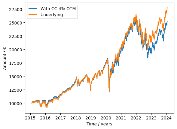
Call Overwriting
This strategy slightly underperformed the underlying, mostly likely due to the strong bull market during this period.
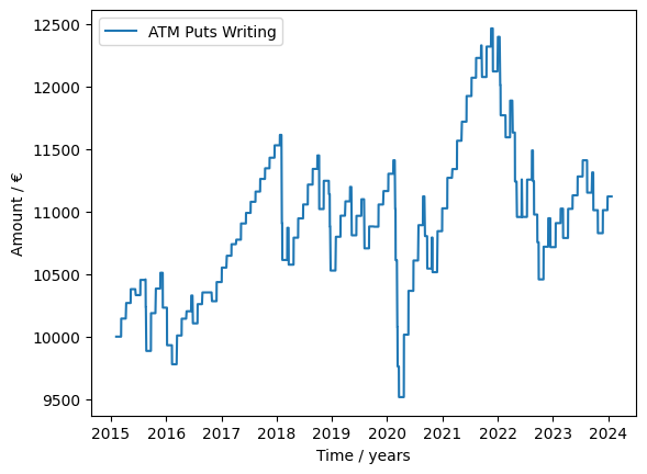
Put writing
Selling ATM Puts returned a small gain, considering this contracts offer a strong hedge, such a small return is unexpected.
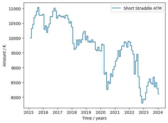
Short Straddle
This strategy shows underperformance during this period. This is a bit surprising since, in general, implied volatility is usually above historical.
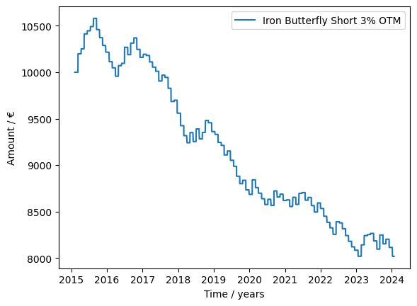
Iron Butterfly
This strategy allows shorting volatility with downside protection. However, it was shown to not be very successful. In fact, the opposite strategy would have performed very well.
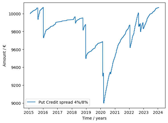
Put credit spread
This strategy was expected to perform well since it gives exposure to Delta and shorts volatility. However, this was not the case.
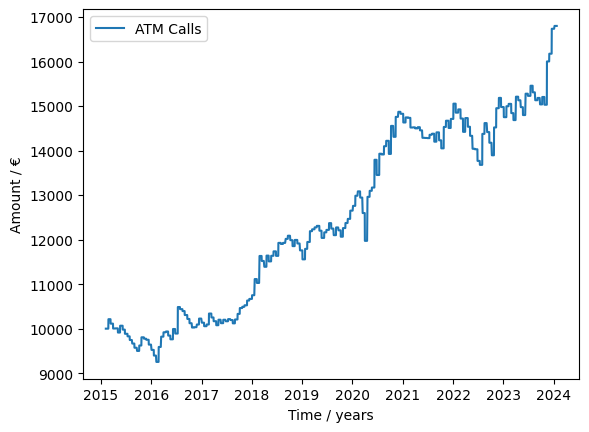
Long ATM Calls
This strategy seems to be the most profitable according to this model. Buying calls offers a position that is both long underlying and volatility which seems to be favorable based on this model.
Conclusion
It is hard to say for sure wether or not the above backtests are reliable, since I do not have access to market data.
Nevertheless, this made me realize how efficient the market is and prevented me from doing blind option plays. So I consider it a success.
Unfortunately it doesn’t allow for more complex strategies such as implementing stop-loss, since this model should be unreliable at calculating prices of contracts with expiration date of less than 30 days.
This being said, I do not recommend implementing a strategy just based on this model. There is high suspicion that this model is biased towards less implied volatility, especially for closer to the money options which is unsurprising since current market conditions are quite stable.
On a brighter note, this model can be used to evaluate how the current option market is priced, especially regarding skew. For example, I can suspect that current skew is low and ATM calls are cheap considering their profitability in this model.